Lane Graph Conditioning for Trajectory Prediction

Abstract

Accurate trajectory prediction for autonomous driving requires understanding both motion dynamics and road structure. While recent learning-based approaches have shown promise, they often struggle to effectively incorporate structured road information, leading to physically implausible predictions that violate lane constraints.

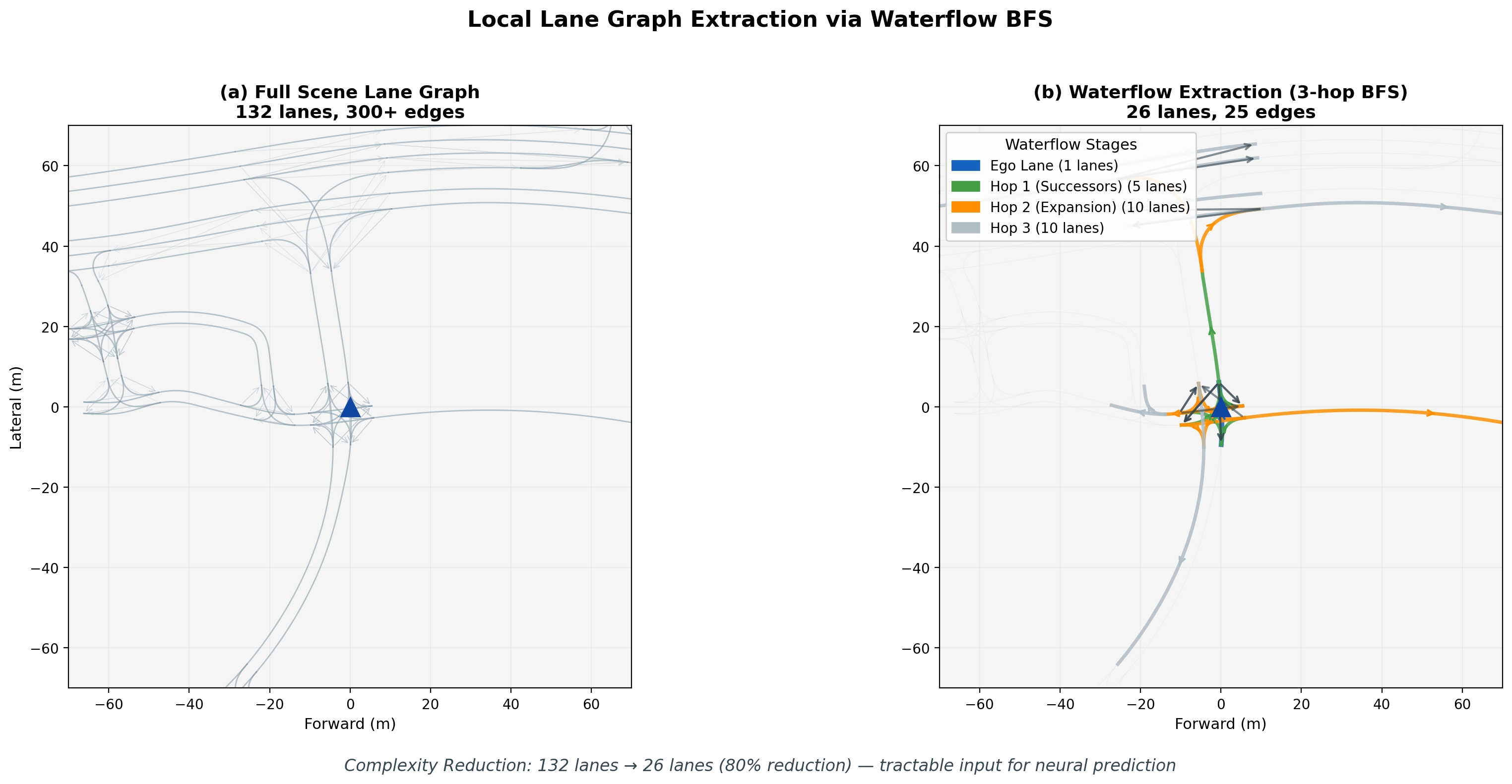
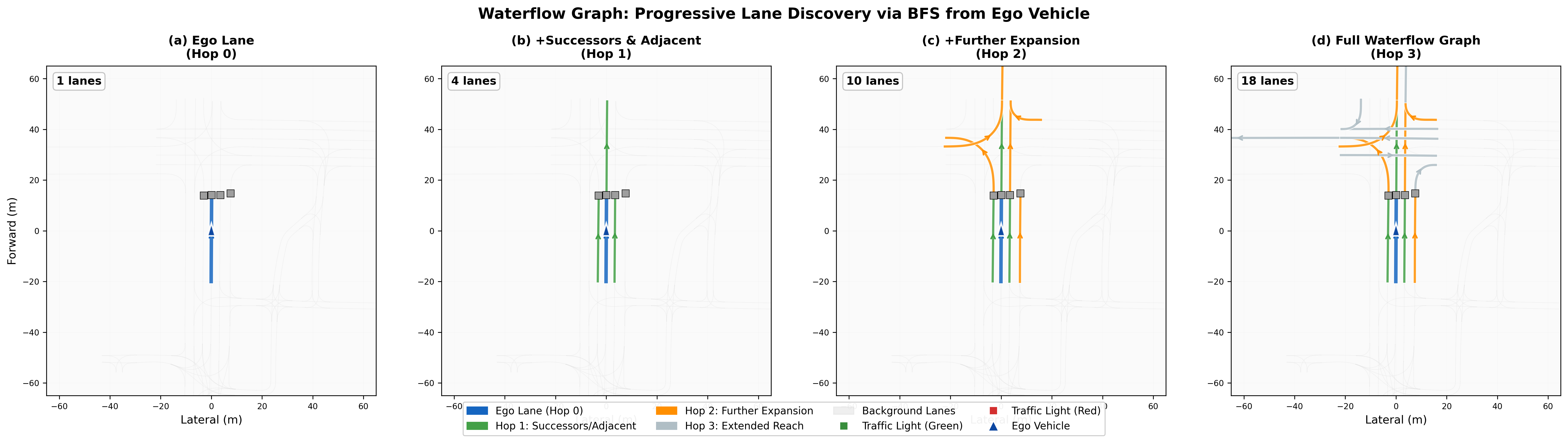
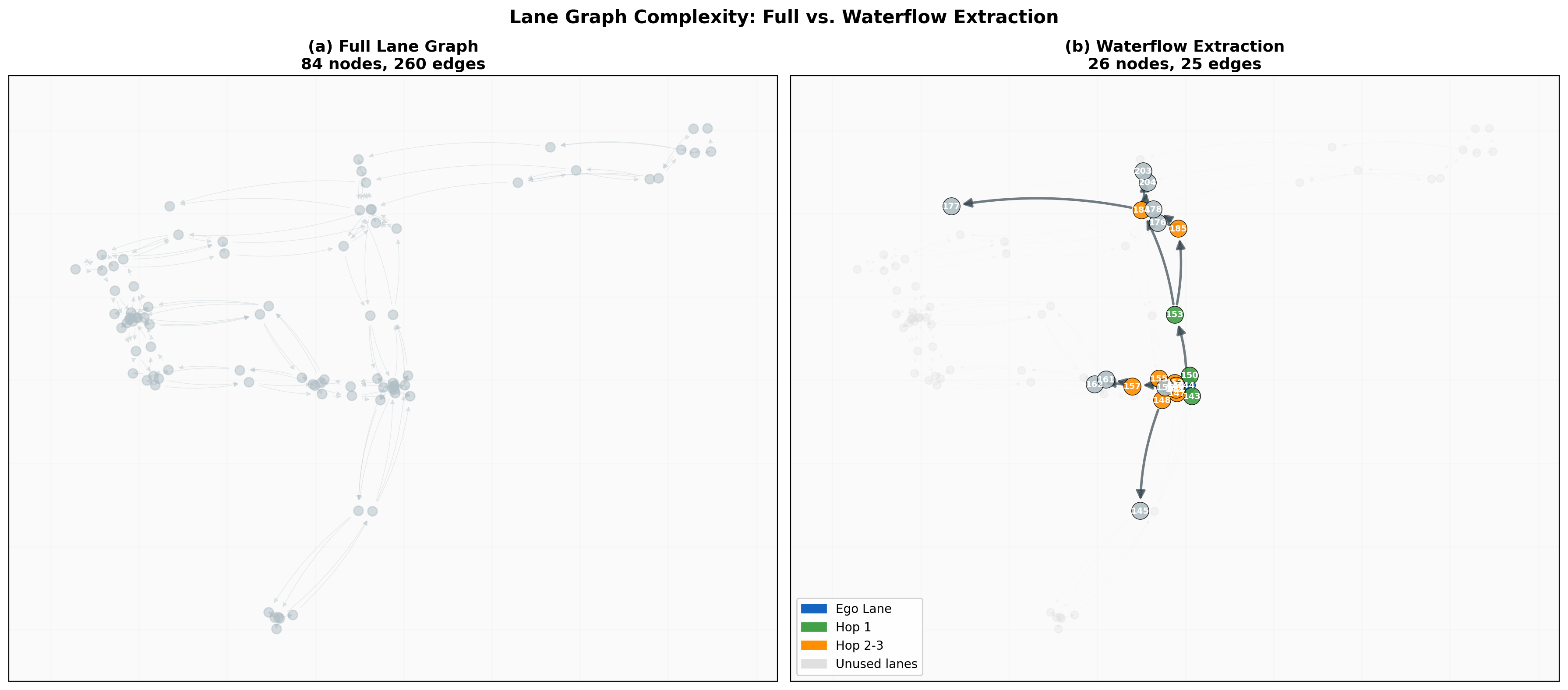
We present a structure-aware trajectory prediction framework that explicitly conditions on local lane graph structure. Our approach introduces a "waterflow" algorithm that extracts a local lane graph via 3-hop breadth-first search from the ego vehicle's current lane, reducing graph size by 80% while preserving critical connectivity information. The extracted lane graph is encoded using graph message passing and fused with trajectory features via cross-attention.

Evaluated on 89,258 signal-controlled intersection scenarios from the Waymo Open Motion Dataset (filtered from 123K processed scenarios, approximately 25% of the 487K WOMD v1.1 training partition), our approach achieves up to 26.7% minADE improvement and 42.7% miss rate reduction in multi-modal prediction. The method is architecture-agnostic, demonstrating consistent gains on both LSTM (+18.7%) and Transformer (+32.0%) backbones. Error decomposition reveals balanced improvements across both longitudinal (+25.4%) and lateral (+26.5%) components, with endpoint lateral error showing the strongest reduction (+30.5%).

26.7%

minADE improvement
(8s, K=6 multi-modal)

42.7%

Miss Rate reduction
(MR@5m: 34.0% → 19.3%)

+47K

Additional parameters
(~8% overhead for LSTM)

2 arch.

Architecture-agnostic
LSTM and Transformer

1.37m

minADE comparable to Waymo
official full-feature LSTM

Key Contributions:

Waterflow Local Lane Graph Extraction: Novel 3-hop BFS algorithm that identifies relevant road structure from the ego lane, achieving 80% graph size reduction while preserving connectivity
Architecture-Agnostic Lane Conditioning: A graph-based lane encoding module with cross-attention fusion that integrates seamlessly into both LSTM and Transformer prediction backbones
Comprehensive Evaluation: Large-scale experiments on 89K Waymo intersection scenes with multi-modal prediction, error decomposition, and cross-architecture validation
Implicit Regularization Effect: We show that lane conditioning acts as an implicit regularizer for Transformer encoders, preventing the overfitting observed in unconditioned models

Multi-Modal Prediction Demos

Side-by-side animated comparison of LSTM Baseline (left half) vs LSTM + Lane Conditioning (right half) on ego-centric bird's-eye view. Each demo shows K=6 multi-modal trajectory predictions growing step-by-step over the 8-second horizon. The lane-conditioned model produces tighter, more lane-aligned trajectories.

Straight-through at intersection
BL: 4.35m → LC: 1.19m (+73%)

Left turn at complex intersection
BL: 8.95m → LC: 3.09m (+65%)

Left turn with lane following
BL: 3.64m → LC: 1.38m (+62%)

Straight-through with neighbors
BL: 1.33m → LC: 0.54m (+59%)

Curved lane following
BL: 1.89m → LC: 0.83m (+56%)

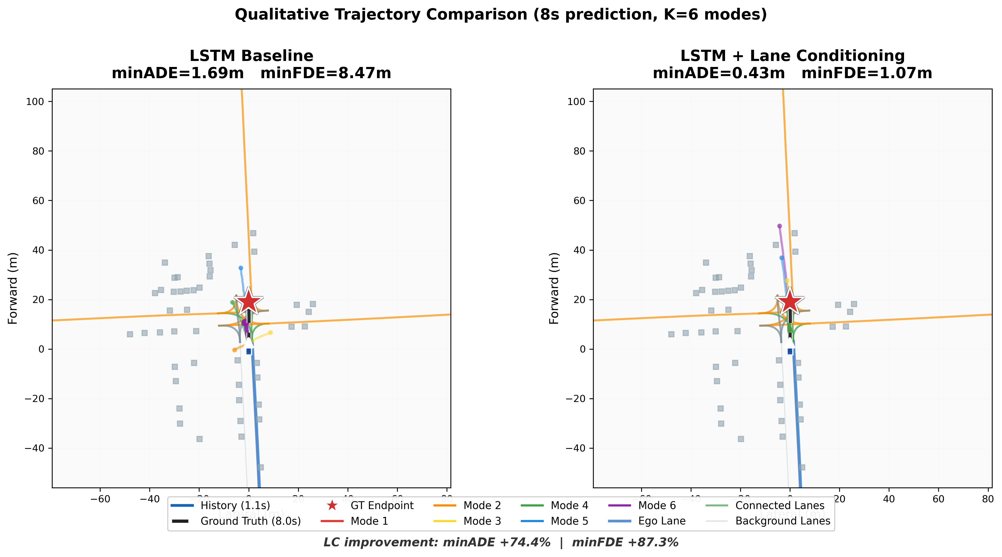
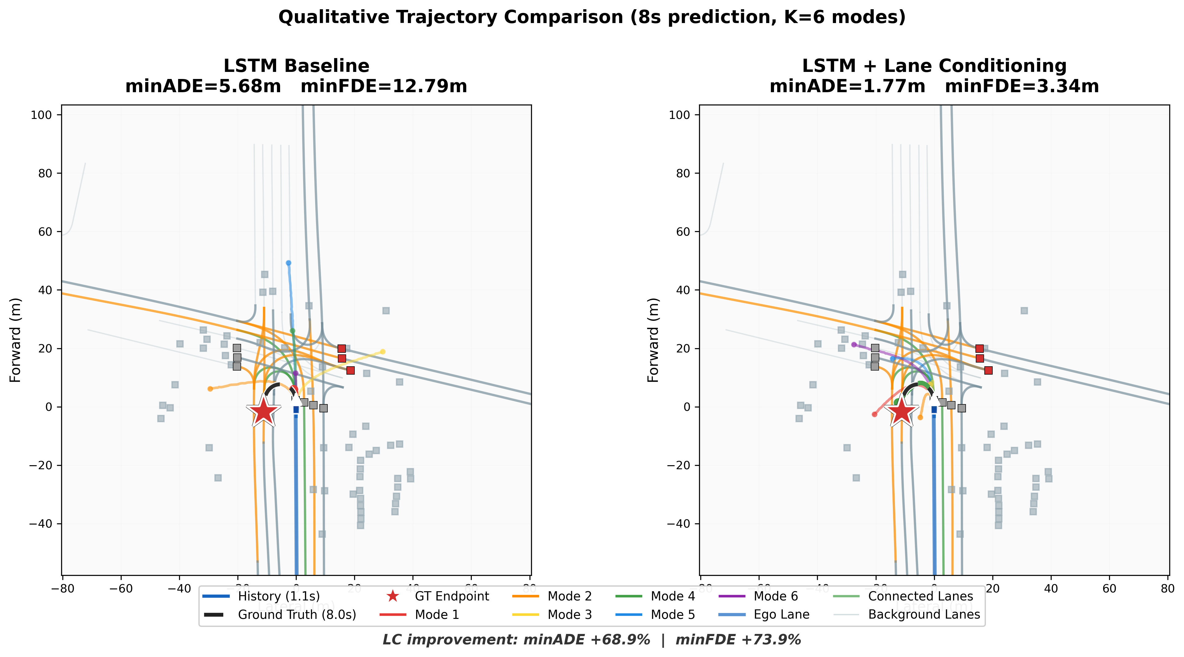
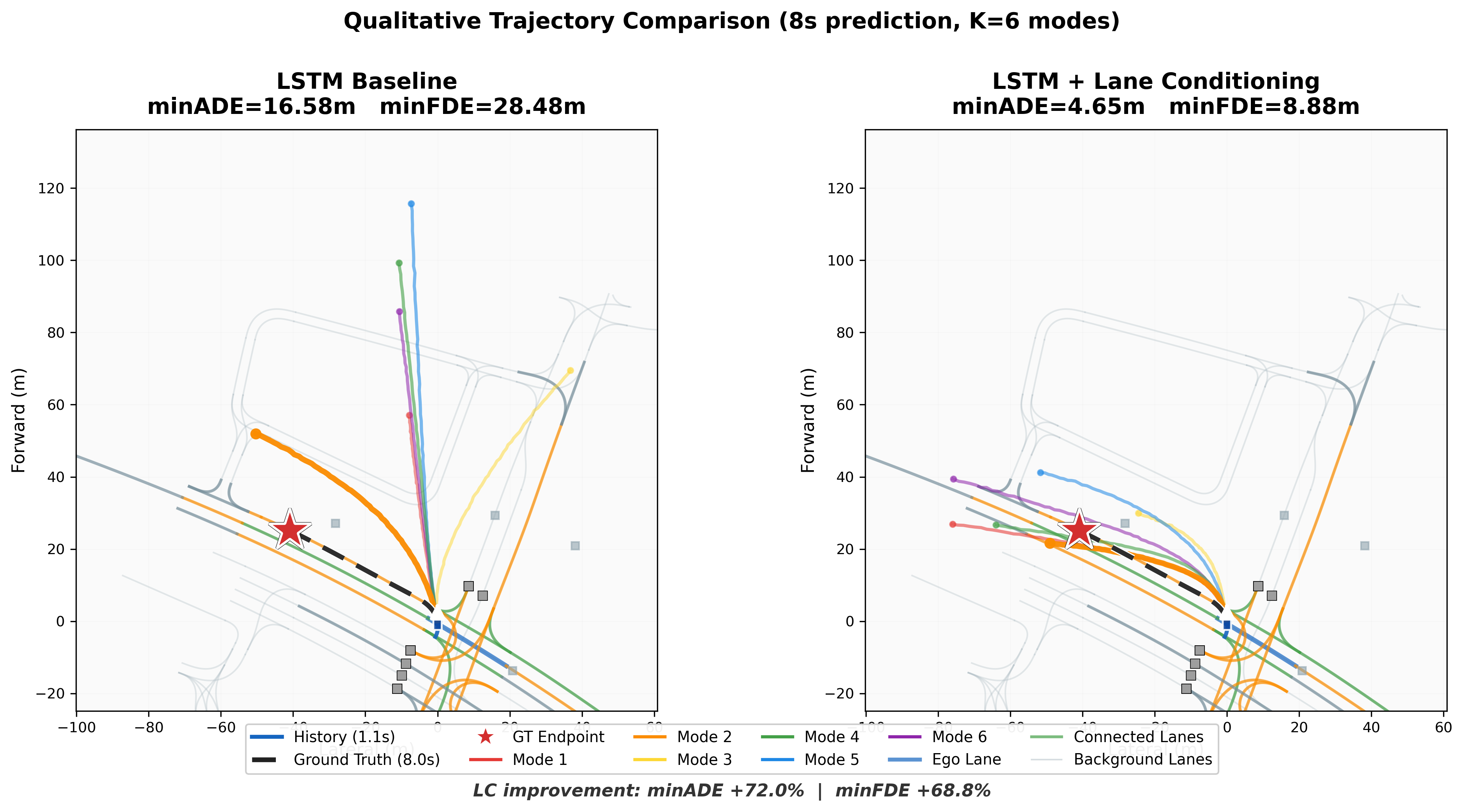
Key observation: The baseline model often spreads predictions across multiple lanes or into off-road areas. Lane conditioning constrains the hypotheses to physically plausible trajectories that follow actual lane geometry, especially at complex intersection turning zones.

Qualitative Trajectory Comparison

Static snapshots comparing all K=6 prediction modes between the baseline and lane-conditioned models. The lane-conditioned model's trajectories follow connected lane structure (shown in green/orange), while the baseline produces scattered, off-road predictions.

Qualitative comparison - straight scenario

Straight-through scenario. The LC model's 6 modes tightly follow the lane structure, achieving minADE 0.43m vs baseline 1.69m (+74.4% improvement).

Qualitative comparison - turning scenario

Turning scenario. LC modes follow the correct turning path along connected lanes, achieving minADE 1.77m vs baseline 5.68m (+68.9% improvement).

Qualitative comparison - complex intersection

Complex intersection with multiple lane options. Even in this challenging case with many possible paths, the LC model reduces minADE from 16.58m to 4.65m (+72.0% improvement).

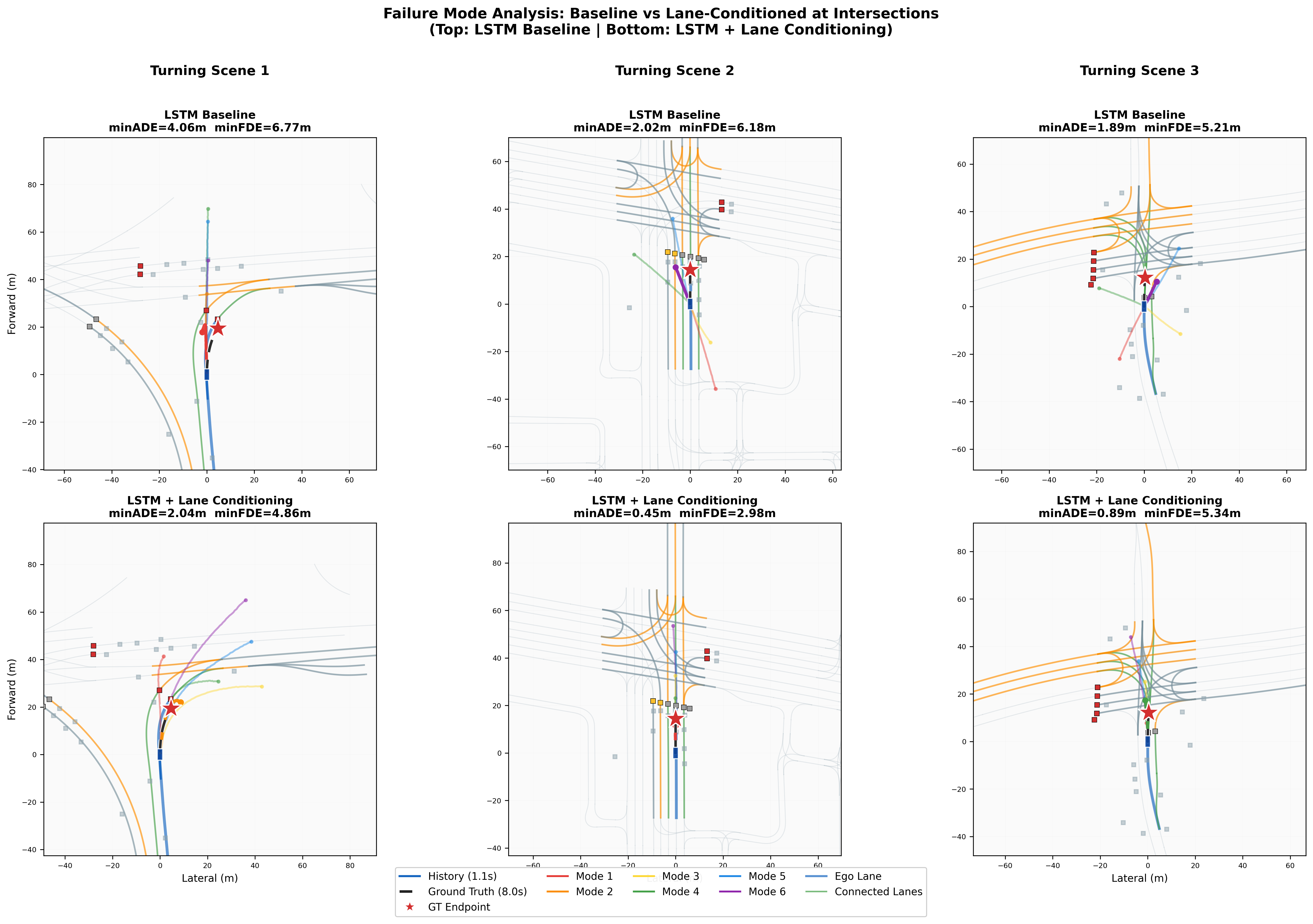
Failure Mode Analysis: Turning at Intersections

The lane-conditioned model shows its greatest advantage during turning maneuvers, where the baseline lacks structural guidance and produces scattered, off-road predictions. These 3 examples show scenes with high ego curvature where BL error is significantly worse than LC.

Failure mode analysis - BL vs LC at turns

Top row: LSTM Baseline. Bottom row: LSTM + Lane Conditioning. At turning scenes, the baseline's K=6 modes scatter across the intersection while the lane-conditioned model aligns predictions to connected lane structure. Best case: BL 4.06m → LC 2.04m (50% reduction).

Rolling Prediction Through Full Scenario

These visualizations sweep the anchor frame through the full 9.1-second scenario, generating a new K=6 multi-modal prediction at each timestep. This shows how predictions evolve as the ego vehicle progresses through the scene. The LC model maintains accurate predictions throughout the entire drive, while the baseline's errors compound over time.

Straight-through (full scenario)
Avg minADE: BL 2.82m → LC 1.21m (+57%)

Turn maneuver (full scenario)
Avg minADE: BL 3.70m → LC 1.66m (+55%)

Straight with lane guidance
Avg minADE: BL 1.03m → LC 0.59m (+43%)

Temporal consistency: The rolling visualization reveals that the lane-conditioned model produces temporally consistent predictions — the trajectory modes smoothly evolve as the vehicle moves, rather than flickering between unrelated hypotheses frame-to-frame.

Numerically Comparable to Waymo Official

Our LC-LSTM using only position + neighbor + lane graph features achieves minADE = 1.37m, comparable to the Waymo official LSTM (1.34m) trained with full kinematic features (velocity, heading, object type, traffic signals, and road graph). This demonstrates that local lane graph conditioning can effectively substitute for hand-engineered features.

1.37m

vs Waymo 1.34m

Experimental Results

We evaluate on 89,258 signal-controlled intersection scenarios selected from the Waymo Open Motion Dataset (WOMD v1.1) training partition. These scenes were filtered from 123K processed scenarios (~25% of WOMD's 487K total training scenarios) to focus on urban intersections with traffic lights, where lane conditioning provides the greatest benefit. We use a custom 85/15 train/val split. All models share the same data pipeline: 1.1s history (11 steps at 10Hz), neighbor encoding, and CV-residual prediction. The lane-conditioned (LC) models additionally receive the local lane graph extracted by the waterflow algorithm.

Short-Horizon Single-Modal Prediction (3s)

To establish statistical significance, we train 3 seeds for 3-second prediction and report mean and standard deviation.

Table 1: 3s single-modal prediction (3 seeds, paired t-test p = 0.0071)
Model	ADE@3s (mean ± std)	Improvement
LSTM Baseline (BL)	0.559 ± 0.007	—
LSTM Lane-Cond (LC)	0.507 ± 0.011	+9.3%

Long-Horizon Single-Modal Prediction (8s)

We extend the prediction horizon to 8 seconds (80 timesteps) and test both LSTM and Transformer backbones. Lane conditioning provides large improvements on both architectures, with Transformer benefiting even more (+32.0% ADE).

Table 2: 8s single-modal prediction (seed42, 100 epochs)
Model	ADE@8s	FDE@8s	ADE@3s	vs Baseline
LSTM-BL	3.781	11.244	0.553	—
LSTM-LC	3.075	8.688	0.516	+18.7%
TF-BL	4.859	13.875	0.828	—
TF-LC	3.303	8.956	0.663	+32.0%

Horizon Scaling: Lane conditioning benefit increases dramatically with prediction horizon: +9.3% at 3 seconds, +18.7% at 8 seconds (LSTM), and +32.0% at 8 seconds (Transformer). This confirms that structural road knowledge becomes increasingly critical for long-range prediction where constant-velocity assumptions break down.

Multi-Modal Prediction (8s, K=6)

For multi-modal prediction, each model generates K=6 trajectory hypotheses per agent. We use the winner-takes-all (WTA) training strategy and report min-of-6 metrics.

Table 3: 8s multi-modal prediction K=6 (3-seed mean ± std)
Model	minADE	minFDE	MR@5m	vs Baseline
LSTM-BL	1.868 ± 0.042	5.047 ± 0.106	34.0 ± 1.3%	—
LSTM-LC	1.371 ± 0.081	3.403 ± 0.242	19.3 ± 0.7%	+26.7% / +32.6% / +42.7%

Multi-Modal Gains: Lane conditioning reduces miss rate from 34.0% to 19.3% — a 42.7% relative reduction. The multi-modal setting amplifies lane conditioning benefits (26.7% minADE improvement vs 18.7% single-modal) because lane structure helps the model generate trajectory hypotheses along distinct lane options (e.g., left turn vs straight vs right turn).

Context: Comparison with Waymo Official Baselines

While not a direct apples-to-apples comparison (different features, evaluation splits), the Waymo Motion Prediction Challenge provides useful context for our results.

Table 4: Context comparison with Waymo official baselines (minADE, 8s, K=6)
Model	Features	minADE (m)
Waymo LSTM (bare)†	Agent state (pos, vel, bbox)	2.63
Our LSTM-BL	Position + Neighbor	1.87
Waymo LSTM + rg + ts + hi†	Agent state + map + signals + interactions	1.34
Our LSTM-LC	Position + Neighbor + Lane	1.37 ± 0.08

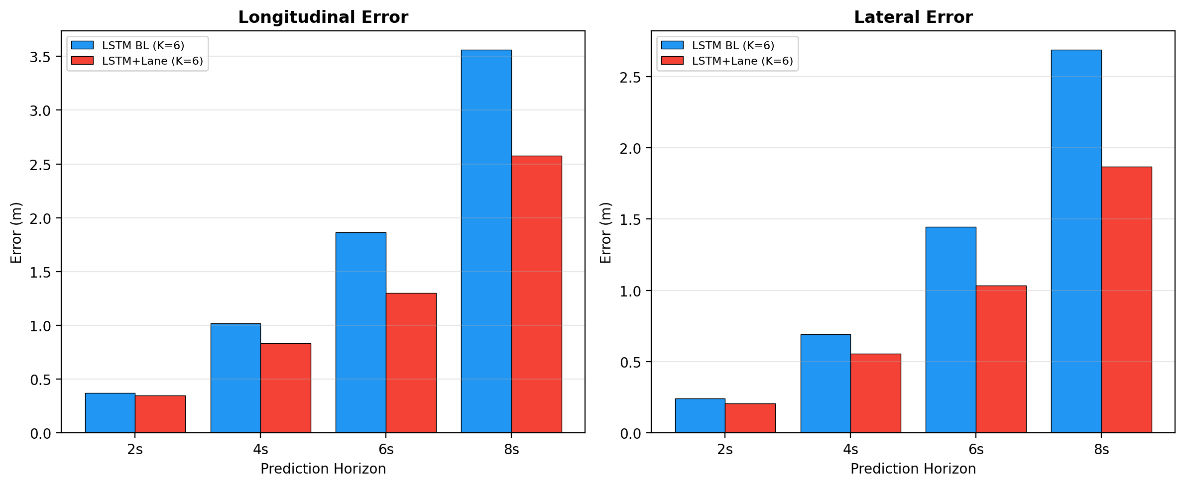
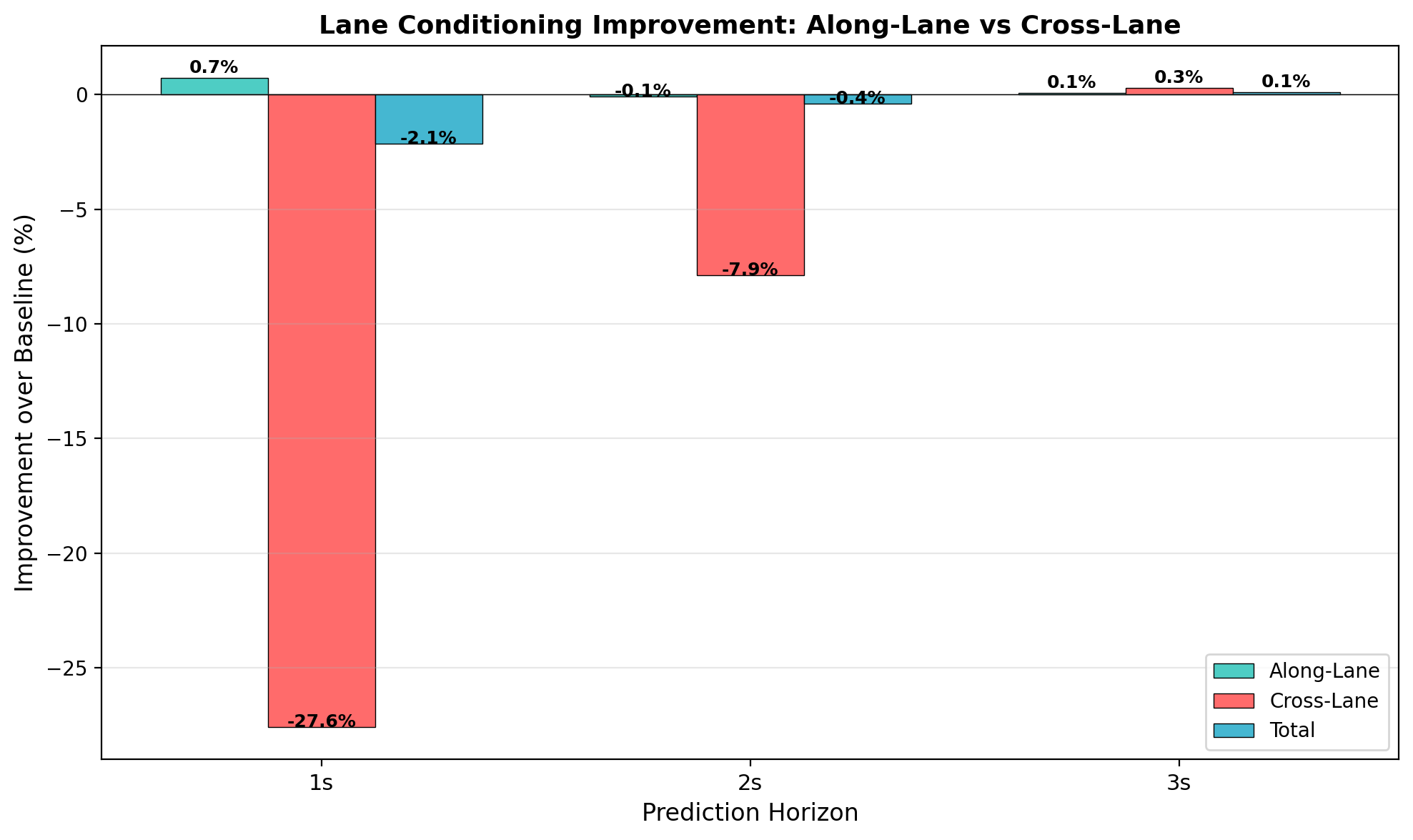
Note: Our LC-LSTM with only position + lane features is numerically comparable to the Waymo official full-feature LSTM (minADE = 1.37m vs Waymo's 1.34m), demonstrating that local lane graph conditioning can effectively substitute for hand-engineered kinematic features. †Waymo baselines from Ettinger et al. (2021), Table 2 (vehicle class, standard val set). Our results use a custom signal-controlled subset with 85/15 split, so values are not directly comparable.

Error Decomposition Analysis

To understand where lane conditioning provides its benefits, we decompose prediction error into longitudinal (along-lane direction) and lateral (cross-lane direction) components for both average and endpoint errors.

Table 5: Error decomposition (8s, K=6 multi-modal)
Component	Baseline (m)	Lane-Cond (m)	Improvement
Average Longitudinal	1.238	0.924	+25.4%
Average Lateral	0.919	0.675	+26.5%
Endpoint Longitudinal	3.561	2.577	+27.6%
Endpoint Lateral	2.687	1.867	+30.5%

Longitudinal vs Lateral Error Comparison

Longitudinal and lateral error by horizon. Lane conditioning reduces both components, with the gap widening at longer horizons.

Improvement percentage over the prediction horizon. Benefits are minimal at 1s but grow to 25–30% by 8s, confirming the horizon scaling effect.

Figure: Total, longitudinal, and lateral error growth over the 8-second horizon. Lane conditioning achieves consistently lower error across all components, with the gap widening at longer horizons where lane structure matters most.

Error decomposition timeline: detailed per-timestep error for all components.

Improvement breakdown by error component. Endpoint lateral error shows the largest improvement (+30.5%), confirming that lane conditioning helps maintain correct lane assignment over long horizons.

Analysis: Lane conditioning provides balanced improvements across both error axes, contrary to an initial hypothesis that it would primarily reduce lateral (cross-lane) error. The strongest individual gain is on endpoint lateral error (+30.5%), which aligns with the intuition that lane structure is most critical for determining the final lane assignment at the end of the 8-second horizon. The substantial longitudinal improvement (+25.4%/+27.6%) suggests that lane geometry also informs speed profile estimation.

Method Overview

Our framework adds a lane conditioning module to a standard trajectory prediction pipeline. The key design principle is architecture-agnostic fusion: the lane encoder communicates with the trajectory encoder through cross-attention, making it compatible with any backbone.

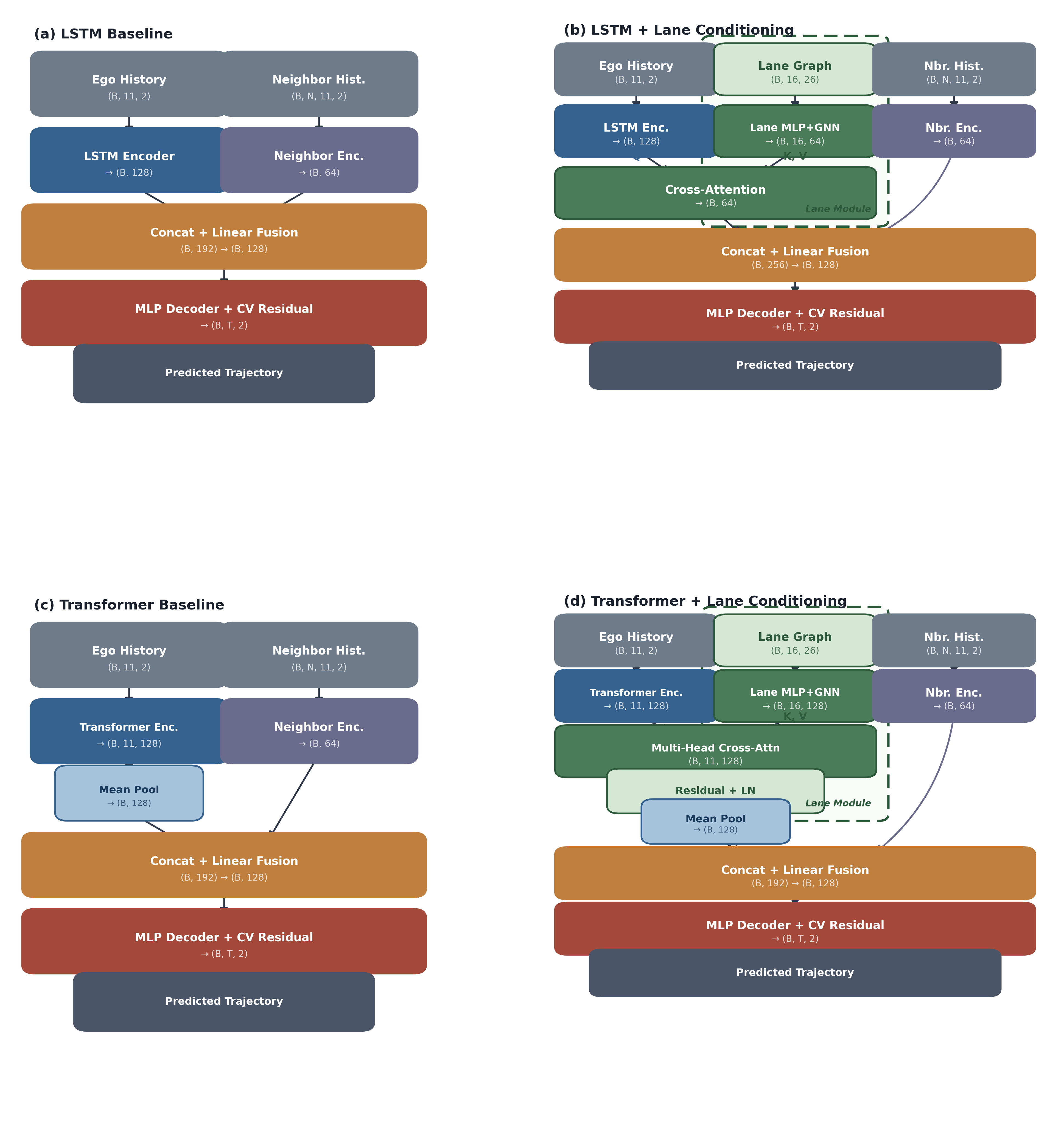
Model architecture overview showing all four configurations: (a) LSTM Baseline, (b) LSTM + Lane Conditioning, (c) Transformer Baseline, (d) Transformer + Lane Conditioning. The lane graph is processed through MLP + graph message passing, then fused with trajectory encoding via cross-attention. The architecture is agnostic to the choice of trajectory encoder.

1. Trajectory Encoder (LSTM / Transformer)

Encodes the observed trajectory history (1.1 seconds, 11 timesteps at 10Hz). LSTM variant: compresses history into a single hidden vector (B, 128). Transformer variant: 2-layer, 4-head self-attention with learnable positional embeddings.

2. Lane Graph Encoder (MLP + Message Passing + Cross-Attention)

Lane Feature Extraction: Each lane segment is encoded using an MLP that processes polyline points, traffic light states, and lane types.

Graph Message Passing: 2 rounds of message passing propagate information through lane connectivity (predecessors, successors, left/right neighbors).

Cross-Attention Fusion: Lane embeddings attend to trajectory features to select the most relevant structural context for the current motion.

3. Neighbor Encoder (LSTM + Max-Pool)

Encodes surrounding vehicles' trajectories using per-neighbor LSTMs, then aggregates via max-pooling to create a permutation-invariant neighbor representation.

4. Fusion + MLP Decoder with CV-Residual Prediction

Fuses trajectory, lane, and neighbor embeddings through concatenation followed by MLP layers. The decoder predicts residuals relative to a constant velocity baseline. For multi-modal prediction, K=6 heads generate diverse trajectory hypotheses trained with winner-takes-all loss.

Parameter Overhead: The lane conditioning module adds only +47K parameters (~8%) for LSTM and +152K parameters (+33.3%) for Transformer backbones.

Waterflow Local Lane Graph Extraction

A key challenge in lane-conditioned prediction is managing the complexity of full road graphs. Real-world intersections can contain dozens of lane segments, most of which are irrelevant to the ego vehicle's near-future trajectory.

Local Lane Graph Extraction via Waterflow BFS. (a) Full scene lane graph with 132 lanes and 300+ edges is too complex for neural prediction. (b) Waterflow 3-hop BFS extracts 26 lanes and 25 edges — an 80% reduction — while preserving all relevant turn options and lane connectivity.

Waterflow concept: starting from the ego lane (red), 3-hop BFS explores along lane connectivity

Extracted graph topology showing lane nodes and connectivity edges (predecessors, successors, neighbors)

Why 3 hops? At a typical intersection with ~4 lane widths per road, 3 hops from the ego lane is sufficient to reach all reachable lanes within the 8-second prediction horizon at typical urban speeds (30–50 km/h). More hops would include irrelevant distant lanes, while fewer would miss important turn options.

Key Findings

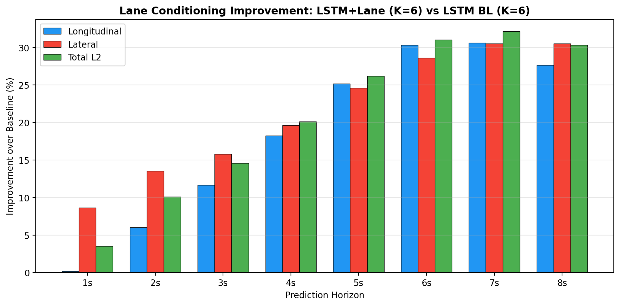
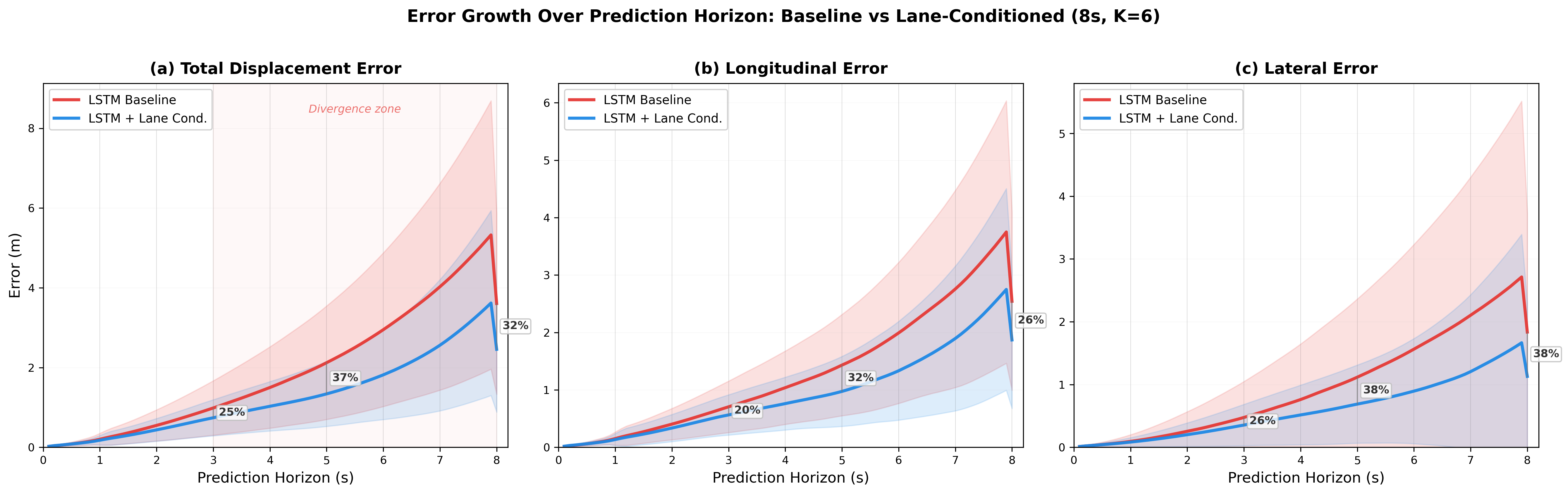
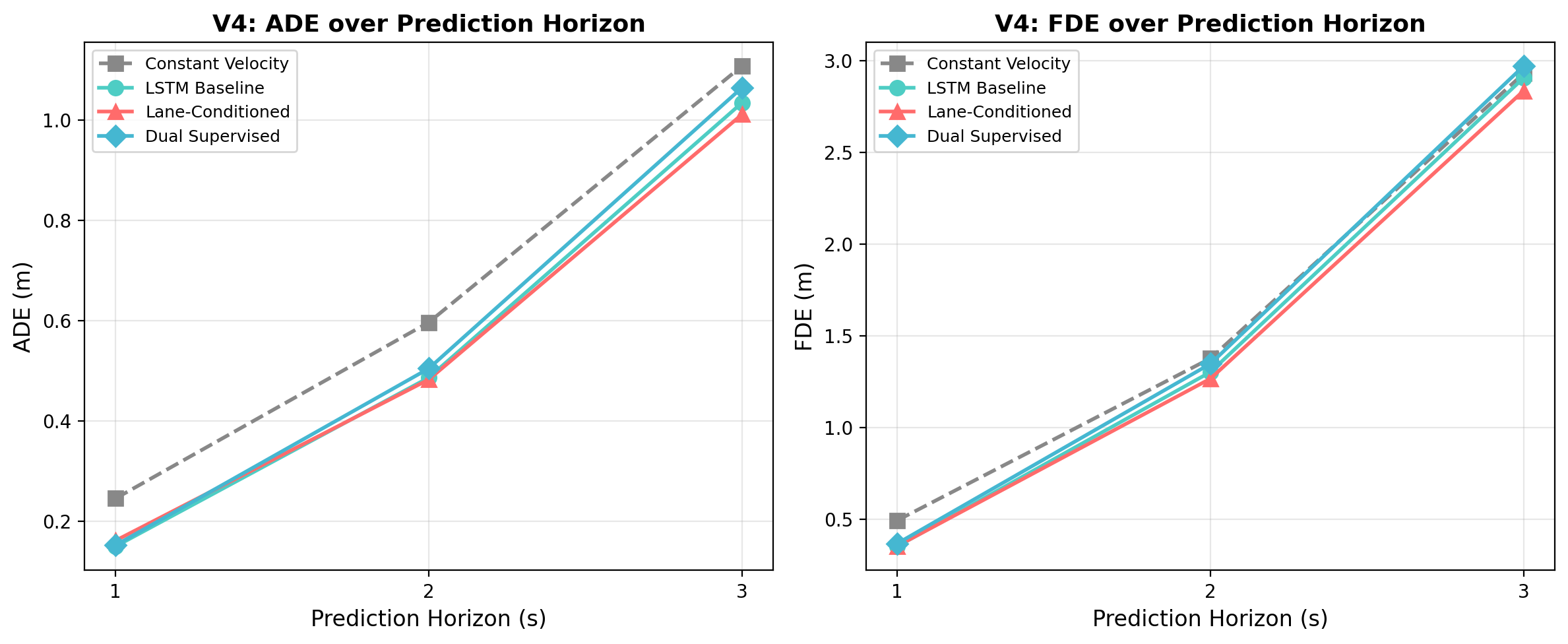
1. Benefit Increases with Prediction Horizon

Lane conditioning becomes increasingly valuable as the prediction horizon grows. At 3 seconds, constant-velocity extrapolation is a reasonable approximation. At 8 seconds, vehicles may change lanes, turn at intersections, or follow curved roads.

Horizon	Setting	Improvement (ADE)
3s	Single-modal, LSTM	+9.3%
8s	Single-modal, LSTM	+18.7%
8s	Multi-modal K=6, LSTM	+26.7%

2. Architecture-Agnostic: LSTM and Transformer

Both LSTM and Transformer encoders benefit substantially, with Transformer showing an even larger relative gain (+32.0% vs +18.7%). Lane conditioning acts as an implicit regularizer for the Transformer — TF-BL overfits severely (ADE 4.859), while TF-LC achieves ADE 3.303.

3. Balanced Error Reduction

Error decomposition reveals improvements in both longitudinal and lateral prediction. The strongest gain is on endpoint lateral error (+30.5%).

4. Delayed Convergence, Lower Asymptote

The lane-conditioned model converges more slowly than the baseline (optimum around epoch 94 vs epoch 23 for baseline). Short training runs can be misleading — 100 epochs is essential to observe the full benefit.

Prediction error growth over the horizon. Lane conditioning achieves consistently lower error, with the gap widening at longer horizons.

5. Numerically Comparable to Waymo Official

Our LC-LSTM achieves minADE = 1.37 ± 0.08m using only position + lane features, comparable to the Waymo official LSTM baseline (1.34m) that uses the full feature set (velocity, heading, object type, etc.).

Additional Analysis

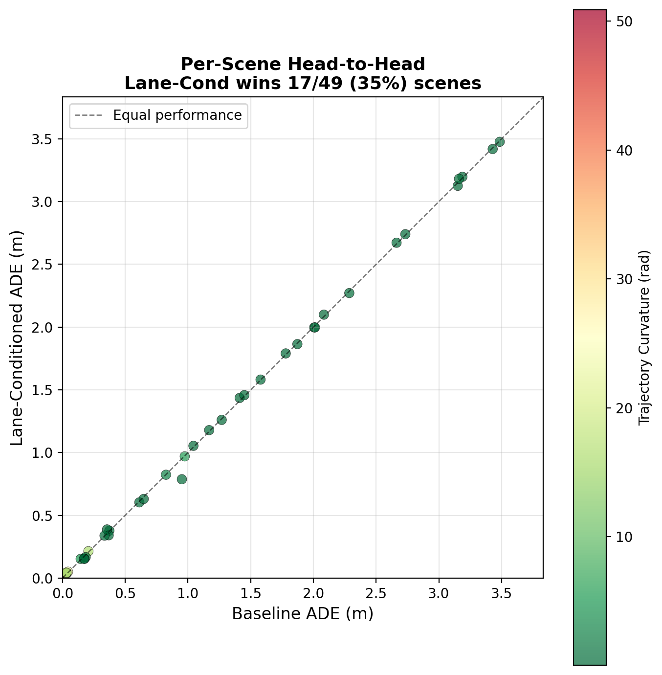
Scene Difficulty Analysis

Lane conditioning improvement by scene difficulty. The benefit is most pronounced on challenging scenarios where vehicles deviate significantly from constant-velocity prediction.

Per-scene head-to-head comparison. Points below the diagonal indicate scenes where lane conditioning outperforms the baseline. The majority of points fall well below the diagonal, confirming consistent improvement.

Dataset

We use the Waymo Open Motion Dataset (WOMD) v1.1 training partition, which contains approximately 487,000 total training scenarios. Our processing pipeline extracts ego vehicle trajectories from each scenario:

Processing Pipeline

Step 1: Extract ~123K scenarios from WOMD training set (~25% of total) and process raw protobuf data into per-scene trajectory and lane graph files.

Step 2: Filter for signal-controlled intersection scenarios, yielding 89,258 scenes with traffic lights. These intersections have the richest lane structure and are where lane conditioning provides the greatest benefit.

Step 3: Split into 85% training / 15% validation using a fixed random seed for reproducibility.

Data Format

Each scene spans 9.1 seconds at 10Hz (91 frames). We use 1.1s (11 frames) as history and predict the remaining 8.0s (80 frames) for multi-modal evaluation, or 3.0s (30 frames) for short-horizon evaluation. All positions are in ego-centric BEV coordinates with forward = up.

Local Lane Graph Conditioning as a General Inductive Bias for Trajectory Prediction